- Setting up
- Load Image & measurements
- Calculate the Line at Infinity
- Affine rectified image
- Measure Coordinates Again
- Calculate the homography
- Composing the transformation
This post is a not about the way to remove the perspective of the image.
Setting up
I used Python to perform the task. I used the following libraries.
import cv2
import numpy as np
from PIL import Image
import matplotlib.pyplot as plt
Load Image & measurements
With the Image module from library Pillow (PIL), it is very easy to load an image as a Python object or numpy array.
img = np.array(Image.open('cam-1-calib.tiff').convert("L"))
We need to measure several points on the image, to get two different parallel lines and orthogonal lines. Thanks to the nature of the picture (it is a chessboard grid), measureing some grid points would do the trick.
px, p1, p2, p3, py, pz = np.array([  # manually measured grid points
    [1335.083, 495], [1411.500, 880.625], [1042.562, 504.375],
    [1059.344, 894.500], [1052.375, 735.562], [1381.000, 723.833]
])

points = [px, p1, p2, p3, py, pz]
name = ["x", "1", "2", "3", "y", "z"]

for n,p in zip(name, points):
    plt.scatter(*p, color='r', marker='x', lw=2, s=72)
    plt.text(*p, n, color='r', fontsize=24)

plt.imshow(img)
plt.xlim(900, 1500)
plt.ylim(400, 1000)
plt.show()
This picture is the ouput of the above code block.
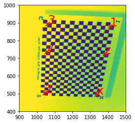
The line connecting point 1 and point 3 ($\mathbf{l} _ {13}$) is parallel to the line connecting point y and point z ($\mathbf{l} _ {yz}$). Similarilly, we have the following relationships.
\[\begin{aligned} \mathbf{l}_{13} &\parallel \mathbf{l}_{yz} \parallel \mathbf{l}_{2x} \\ \mathbf{l}_{32} &\parallel \mathbf{l}_{1x} \\ \mathbf{l}_{32} &\perp \mathbf{l}_{2x} \\ \mathbf{l}_{xy} &\perp \mathbf{l}_{z2} \\ \end{aligned}\]Calculate the Line at Infinity
The following code block calculate the line at infinity ($\mathbf{l} _ {\infty}$), which will be used to recorve the information about parallel lines in the image.
pxh, p1h, p2h, p3h = [np.hstack((p, 1)) for p in (points[:4])]
l13 = np.cross(p1h, p3h)
l2x = np.cross(p2h, pxh)
l1x = np.cross(p1h, pxh)
l23 = np.cross(p2h, p3h)

p_inf_1h = np.cross(l13, l2x)
p_inf_1 = (p_inf_1h / p_inf_1h[-1])[:2]
p_inf_2h = np.cross(l1x, l23)
p_inf_2 = (p_inf_2h / p_inf_2h[-1])[:2]

plt.imshow(img)
plt.scatter(*p_inf_1, color='k')
plt.scatter(*p_inf_2, color='k')
plt.plot(*np.vstack((p_inf_1, p_inf_2)).T, color='k')
plt.show()

l_inf = np.cross(p_inf_1h, p_inf_2h)
l_inf = l_inf / l_inf[-1]
print(l_inf)
The out put image is below. The $\mathbf{l} _ {\infty}$ is very far away from the image (which is a small yellow patch).

This is the homogeneous representation of $\mathbf{l} _ {\infty}$.
[-2.60516041e-06 7.16055835e-04 1.00000000e+00]
Affine rectified image
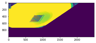
- If we apply the transformation obtained from $\mathbf{l} _ {\infty}$, we get a new image
- In such image, parallel line in real life is parallel in the image
H = np.vstack(([1, 0, 0], [0, 1, 0], l_inf))
affine = cv2.warpPerspective(img, H, (2500, 1000))
plt.imshow(affine)
plt.show()
plt.close()
img_affine = Image.fromarray(affine)
img_affine.save('cam-1-calib-affine.png')
img_affine.close()
This is the result. In this image all the parallel lines are parallel now.
Measure Coordinates Again
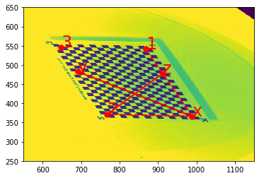
- Now we want to recover such information: perpendicular lines in real life should be perpendicular in the image
- This is to say, we want our image to be the result of, not an affine transformation, but a similar transformation.
- We do this by specifying two perpendicular pairs in the image. In this case, it is $\mathbf{l} _ {x1}$ & $\mathbf{l} _ {x2}$; and also $\mathbf{l} _ {2z}$ & $\mathbf{l} _ {3y}$.
The following code demonstratethe calculation procedure.
points_A = list(map(
    lambda x: H @ np.hstack((x, 1)), points
))
points_A = np.array([p/p[-1] for p in points_A])
px_Ah, p1_Ah, p2_Ah, p3_Ah, py_Ah, pz_Ah = points_A
names_A = ['x', '1', '2', '3', 'y', 'z']

for p, n in zip(points_A, names_A):
    plt.scatter(*p[:2], color='r', marker='o', lw=2, s=42)
    plt.text(*p[:2], n, color='r', fontsize=24)

plt.plot(*np.vstack((px_Ah[:2], p1_Ah[:2])).T, '--', color='r', lw=2)
plt.plot(*np.vstack((px_Ah[:2], p2_Ah[:2])).T, '--', color='r', lw=2)

plt.plot(*np.vstack((px_Ah[:2], py_Ah[:2])).T, color='r', lw=2)
plt.plot(*np.vstack((p2_Ah[:2], pz_Ah[:2])).T, color='r', lw=2)

plt.imshow(affine)
plt.xlim(550, 1150)
plt.ylim(250, 650)
plt.show()
The image illustrates the measurement results. Notice that the perpendicular lines (in real life) are not perpendicular in the image.
Calculate the homography
The following code calculate the homography from the affine image to similar image.
# first orthogonal pair, x1 & x2
lx2_Ah = np.cross(px_Ah, p2_Ah)
lx1_Ah = np.cross(px_Ah, p1_Ah)
lx2_A = (lx2_Ah / lx2_Ah[-1])[:2]
lx1_A = (lx1_Ah / lx1_Ah[-1])[:2]

# second orthogonal pair, 2z & xy
l2z_Ah = np.cross(p2_Ah, pz_Ah)
lxy_Ah = np.cross(px_Ah, py_Ah)
l2z_A = (l2z_Ah / l2z_Ah[-1])[:2]
lxy_A = (lxy_Ah / lxy_Ah[-1])[:2]

# Solve for M(2, 3) * S(3, 1) == 0
M = np.empty((2, 3))

m, l = lx1_A, lx2_A
M[0][0] = m[0]*l[0]
M[0][1] = m[0]*l[1] + m[1]*l[0]
M[0][2] = m[1]*l[1]

m, l = l2z_A, lxy_A
M[1][0] = m[0]*l[0]
M[1][1] = m[0]*l[1] + m[1]*l[0]
M[1][2] = m[1]*l[1]

s11, s12 = np.linalg.solve(M[:, :2], -M[:, -1])

S = np.array([
    [s11, s12],
    [s12, 1],
])  # we set s22 to be 1

S = S / max(s11, 1)  # force image to be expanded

K = np.linalg.cholesky(S)  # affinity component K in the bible
HA = np.array([
    [K[0, 0], K[0, 1], 0],
    [K[1, 0], K[1, 1], 0],
    [0, 0, 1],
]) # Homography for Affinity

similar = cv2.warpPerspective(affine, np.linalg.inv(HA), (2500, 2500))
plt.imshow(similar)
plt.show()

img_similar = Image.fromarray(similar)
img_similar.save('similar.png')
The result is the following image. Look at the fact that the chessboard obtains its origional rectangular shape now, which means the perspective is removed effectively.
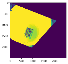
- Notice the result is NOT equivelant to an image taken from a top view, even though it looks very similar. (Image from the top view is still a projective transformation)
- It is the similar transformation of the plane of the chessboard. In real 3D space, the distances and angles are not invariant if they were not on the same plane of the chessboard.
Composing the transformation
In the end we get the matrix Hs that transforms a projective image to a similar image
Hs = np.linalg.inv(HA) @ H
fish = np.array(Image.open('cam-1.png').convert("L"))

fish = cv2.warpPerspective(fish, Hs, (2500, 2500))
plt.show()

img_fish = Image.fromarray(fish)
img_fish.save('cam-1-fish.png')